Introduction

We would like to control our system. And we will walk through this control in the simple case of intensity control, which is a very straight-forward example, which allows us to understand the basics.

Terminology and Basics

This section closely follow ideas from (Citation: Bechhoefer, 2005) Bechhoefer, J. (2005). Feedback for physicists: A tutorial essay on control. Reviews of Modern Physics, 77(3). 783–836. https://doi.org/10.1103/revmodphys.77.783 . A generic feedback control is seen in Fig. 1. A system $G(s)$ is being controlled with a control signal $r(s)$. The goal of the feedback is for the output of the system $y(s)$ to follow the control signal $r(s)$. The general idea is the following: measure the output of the system, determine its difference to the control voltage to get error $\epsilon$ and use this error signal as input for some control law $K(s)$ that tries to minimize the error signal.

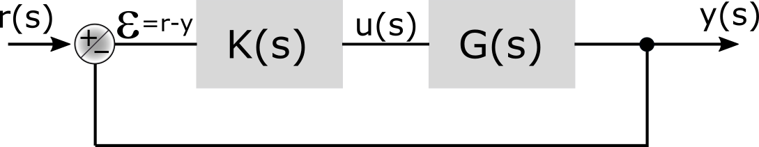
Here we analyze the system in frequency space, where $s=i\omega$. This is a convenient way to analyze control systems. An easy way to measure quantity of such a system is the closed-loop transfer function $T$:

$$T= \frac{y(s)}{r(s)} = \frac{K(s)G(s)}{1+K(s)G(s)}$$

For system stability the loop-shape $H$ is important and can be determined from $T$: $$ H = K(s)G(s) = \frac{T}{1-T} \tag{1} \label{1} $$ Why is it important ? As we see from (\ref{1}), the system gets unstable if $KG= -1$. This means that a feedback system will get unstable if $|KG|=1$ with a simultaneous phase lag of 180°.

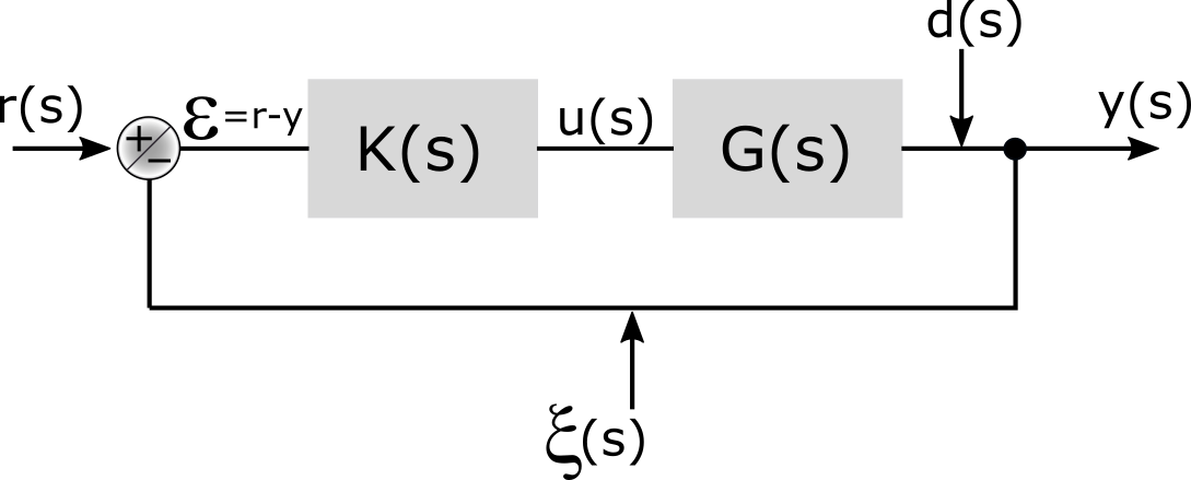
Whereas it is good to have control over an output variable up to a certain frequency, we are in many cases also interested in noise suppression. For example, atoms in a dipole trap experience a heating rate proportional to intensity fluctuations at twice the trap frequency. Only by suppressing the laser intensity noise, you can assure long trap lifetimes and/or ground state atoms. For this reason we consider output disturbances $d(s)$ and sensor noise $\xi (s)$ (see Fig. 2):

$$ y(s) = \frac{KG}{1+KG}[ r(s)-\xi(s)] + \frac{1}{1+KG}d(s) $$

What does this mean? There are two things to learn from that. Let’s start with the disturbances, and introduce the sensitivity, sometimes also called noise suppression: $$S = \frac{1}{1+KG} = 1-T$$ We see that a servo with a high gain leads to a low sensitivity to outside disturbances. The trade-off is that the higher the gain, the noisier the output signal. The reason is that with detector noise the control signal effectively becomes $r(s)-\xi(s)$, meaning that we cannot distinguish the control signal from measurement noise. Thus the higher the gain, the noisier the output.

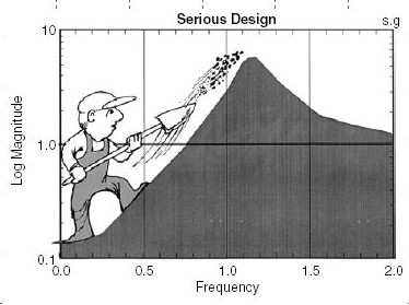
Another trade-off - which holds for almost all systems (to be exact: if KG has at least two more poles than zeros, and has no poles in the right half plane (is stable)) - is the following: $$\int_0^\infty ln|S(s)|ds =0$$ This is known as Bode’s sensitivity integral. It means that if you suppress the Sensitivity to disturbances in some frequency regime, you necessarily increase it in some other frequency regime (see Fig. 3 taken from (Citation: Stein, 2003) Stein, G. (2003). Respect the unstable. IEEE Control Systems Magazine, 23(4). 12–25. https://doi.org/10.1109/mcs.2003.1213600 ).

Now before looking at the different systems $G(s)$, we have a look at the control law $K(s)$. The most-used controller is the PID-controller, or very often experimentally only a PI-controller. The P stands for proportional gain, the I for integral gain and the D for derivative gain. Which makes sense if we look at the response in time domain:

$$u(t) = K_p\epsilon(t) + K_i\int \epsilon(t) dt + K_D \frac{d\epsilon}{dt}$$

In frequency domain the same thing has the following form:

$$K(s) = \frac{u(s)}{\epsilon(s)} = K_p + \frac{K_i}{s} + K_Ds$$

Intensity stabilization

Overview

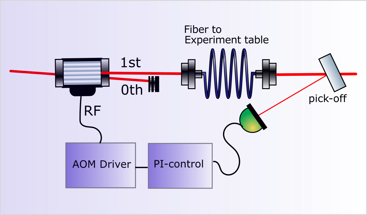
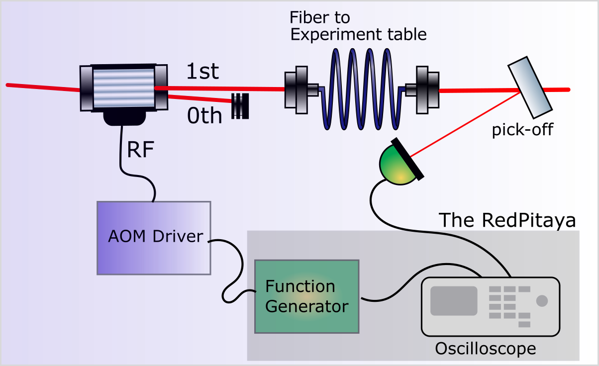
For the control of the intensity, we typically have the set-up that is sketched in Fig. 4. The power of the AOM’s first order beam is dependent on the RF power: $\epsilon_{1st order}\approx\sin^2(P_{RF}/P_{RF_{sat}})$. Therefore the power of the laser beam that leads to the experiment can be controlled by modulating the RF power.

The System

How to characterize the system without PI contol? (“system” refers to AOM+Driver+AOM+Photodiode) The tools needed for that are a function generator, oscilloscope and a network analyzer. All of that can be found in the RedPitaya controlled by PyRPL we use (see Fig. 5).

So what do we measure? As mentioned in the Introduction, we can measure the closed-loop transfer function $T$ and then calculate the open-loop transfer function $H$ to look for a desired loopshape.

How to change laser power by modulating RF power

The whole intensity stabilization is based on being able to modulate the RF power that goes to the AOM. In our case, we have a home-build AOM driver that allows for this modulation with a control voltage ranging from 0 to 1V. Most drivers work with a Voltage Controlled Oscillator, a Mixer or Variable Voltage Attenuator to attenuate the RF power, and and an amplifier end-stage, because the AOM usually requires 30dBm, while the VCO outputs something much lower.

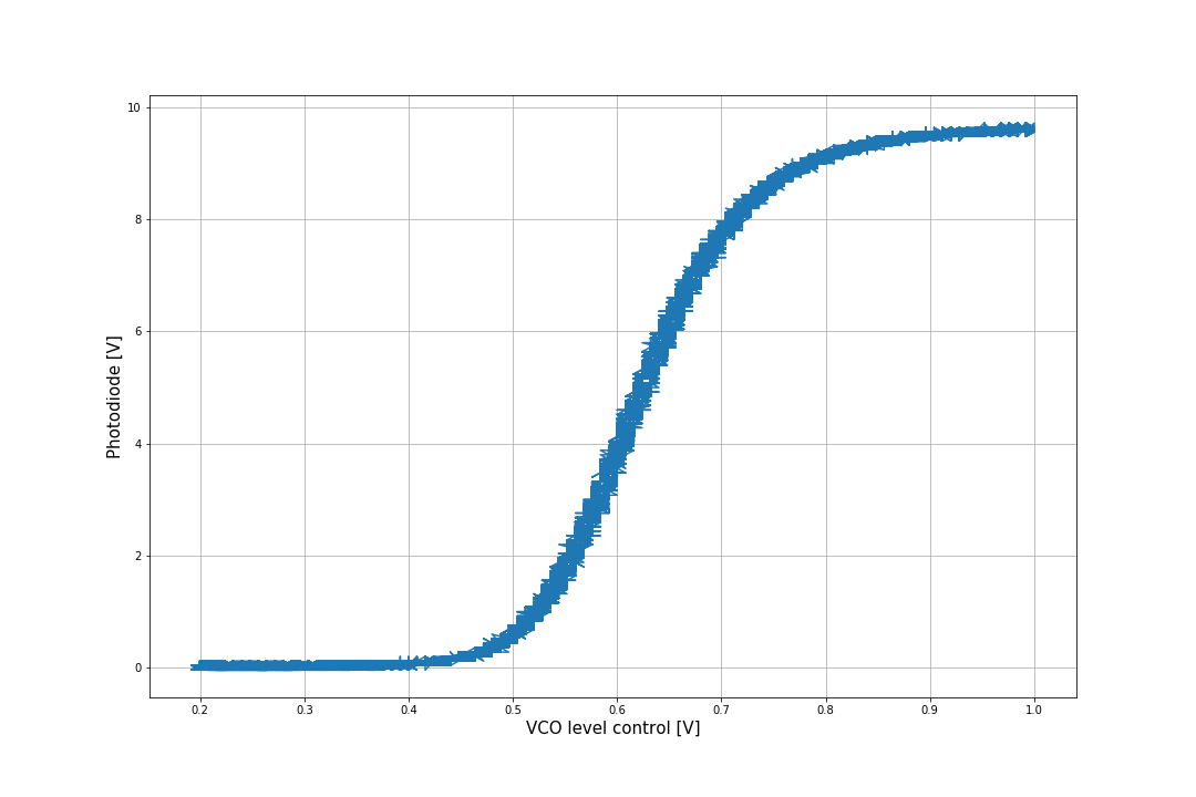
Therefore the voltage on the photodiode depends on the control voltage at the AOM driver and the dependency is nonlinear (see figure 6).

Analysis in Frequency space with Bode plots

The RedPitaya with its network analyzer module, allows us to characterize the setup in frequency space. In the figure above we saw how the Photodiode voltage (laser power) depends on the control voltage on the AOM driver when applying a DC or very low frequency signal. Now we modulate the VCO control voltage with the following: $U_{control}=0.6V+0.01V\cdot\sin\left(2\cdot\pi\cdot f\cdot t\right)$ Can the Photodiode follow this modulation up to arbitrary frequency? Probably not, but how can we measure this? The network analyzer can excite the system with above voltage $U_{control}$ and compare the amplitude of oscillation in the and $U_{Photodiode}$ to measure magnitude and phase. It does so by demodulating the photodiode signal with the same sine that was used for excitation and a corresponding cosine, then lowpass-filtering and averaging the two quadratures for a well-defined number of cycles (see Pyrpl API). From the two quadratures it is now possible to extract the magnitude and phase shift of our system in the probed frequency regime. In the figure below we see that for low frequencies the system follows without phase lag and for higher frequencies the phase increasingly lags as the signal magnitude decreases.

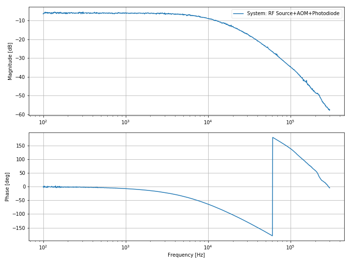
It’s clear that this system doesn’t have any resonances and behaves quiet nicely in the displayed frequency regime. Therefore time-domain tuning methods for a servo like Ziegler-Nichols tuning can be effective and quick. But not every system behaves as nicely as this, so looking at the frequency-regime can be interesting and a way to improve your control, e.g. finding and filtering resonances makes it possible to increase overall gain without sacrificing stability.

A closed loop

After connecting the PI-controller which in our case is also done by the RedPitaya, we close the feedback loop. Now we select some proportional and integral constants such that the intensity is locked to a setpoint we choose. That means that the voltage on the photodetector will be the same as the chosen setpoint. How do we characterize the lock now? How do we know how stable the lock is? How do we know until which frequency noise is surpressed? We take the closed-loop transfer function T using the RedPitaya. With that we can calculate the open-loop transfer function H and look at the sensitivity S.

After measuring T we can can calculate H. As mentioned in the introduction the criterion for instability is $\left|H\right|>1$ for a simultaneously phase lag close to 180°. Be careful that the unit in the figure is dB, which means that $\left|H\right|= 1 = 0 dB$. For low frequencies the transfer functino is ruled by the integrator’s characteristics. Which means high gain, but only a phase lag of 90°.

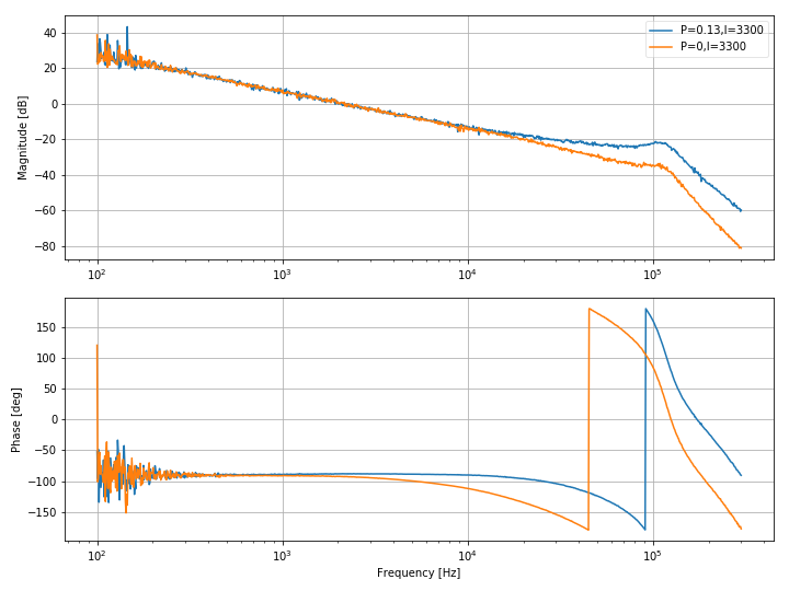
The interesting regime is where the phase lag hits -180° which happens for ~40kHz for the orange curve and ~90kHz for the blue curve. But both sets of P&I-constants lead to stable behaviour, because the magnitude at that point is below 0dB.
The conclusion of this analysis shows that we could have gotten away with a higher proportional or integral constant and still have a stable system.

Sensitivity and noise surpression

At this stage, we can finally analyse the level of noise suppression in the system.

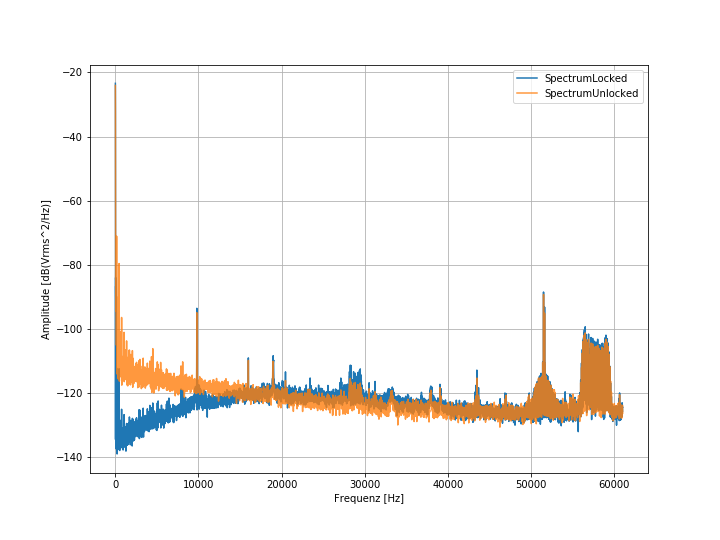
We observe noise suppression for frequencies up to point where the system can react actively, which is about 30kHz.

Further Reading: Problems of Intensity stabilization

Here we can already identify the first pitfall of intensity stabilization. The system, mainly the attenuator inside of the AOM driver, has a proportional gain that depends on the control voltage and is proportional to the slope . The highest gain (slope) is around a control voltage of 0.6V, and the proportional gain for values at 0.4V and 0.9V is very low. On the contrary, the PI-controller has fixed proportional and integral constants.
If you only want one specific laser power in your experiment, this does not bother you. You are using more or less one control voltage that gives you the desired laser power and then you tune the proportional constant of your PI-controller such that the system has the biggest bandwidth.
But imagine you would want to change this laser power now. By choosing a different setpoint/control voltage you would increase/decrease your proportional gain drastically end end up with an oscillating system or a system with very low bandwidth. If you would want your system to be stable for all control voltages, you would have to make sure that for the highest system proportional gain for a control voltage of 0.6V, you choose your PI-controller proportional gain such that your system is stable. Then you have the biggest bandwidth around a control voltage of 0.6V, but for all other control voltages you would have a smaller bandwidth. Imagine the worst case: You want high laser power for loading your laser dipole trap, and then reduce the trap depth for evaporative cooling by decreasing the laser power by a factor of 100. In the Figure this could for example mean, that you have a photodiode voltage of 9V for loading your trap and 90mV for evaporative cooling. In both cases the slope (proportional gain) is very small. If you want your laser power to be stable and not oscillating during the ramp-down (decrease of factor 100), you would have to accept a low bandwidth in both cases, for the loading and the evaporative cooling. One work-around could be that you sacrifice system-stability during the ramp-down for higher proportional gains in the loading and cooling stage. This however could lead to atom-loss due to parametric heating.

Another thing to keep in mind: usually your experimental approach is the following: I want 100mW during the first stage of the experiment and 10mW during the second stage of the experiment. For you to be able to choose a good regime of control voltage values, e.g. 0.5-0.7V, where the AOM Driver gain changes minimally, you have to be able to change either photodiode gain, pick-off ratio or initial laser power.